Introduction
Little's Law deals with averages. It can help us calculate the average waiting time of an item in the system. In project development we break the project delivery into work items. We are interested in how much time it will take for all the items to be processed by the system. And that is what Anderson's formula does - it gives us the relationship between the average lead time for an item and the finite time period over which the project will be delivered.
Little’s Law
Let’s recall what the Little’s Law for production systems is:

Anderson’s Formula
Let’s consider project planning. On Fig.1 we have two levels of the system and hence two perspectives on it:
- Client layer – project or set of customer defined requirements meaningful to the customer.
- Service level – components or work items suitable for the development organization. User stories are just an example of a suitable work item type
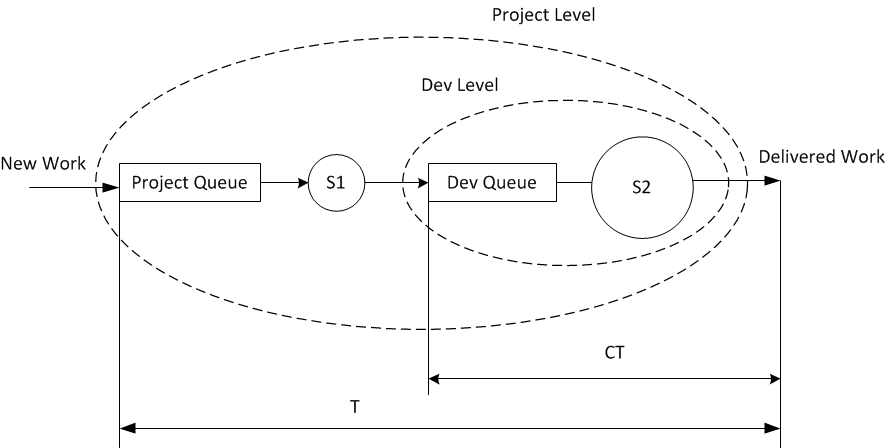
Fig. 1
We can calculate the lead time for the project using the formula:

We can calculate the developers we will need to deliver for a particular lead time using the formula:

Where:
T = time period over which the project will be delivered (lead time)
N = the number of items to be delivered or the total arrivals in [0,T]


Of course THt is the average of a random variable modeled by a distribution of some type. If the departure is a Poisson process with intensity THt then the required time for N-th work item to exit the system (be delivered) is modeled by a Gamma distribution Gamma(a,b) with a=N and b=1/THt.
Proof of Anderson’s Formula
We apply Little’s Law at the client level:


By noting that

It follows that

As well as that

or

Examples
Original example from David Anderson
We have a major project with 2200 user stories to be delivered. The business needs the project delivered in 10 months. The questions to answer are: How much money do we need? How many people do we need?
So we have N = 2200 user stories, T=10 months = 40 weeks. We also have historical data that average lead time for the development organization is 0,4 weeks. Using the Anderson’s formula (2) we have:

The result should be used for the second leg of the Z-curve, but that is another topic.
Calculating delivery date
Let’s have a similar project with major project with 2200 user stories to be delivered. The business wants to know when we will be able to deliver. There are no options for adding more developers to the development organization so we know the average work in process which is 22 user stories. We also have historical data that average lead time for the development organization is 0.4 weeks per user story. Using the Anderson’s formula (1) we have:

The result should be used for the second leg of the Z-curve, but that is another topic.
References:
Little, J. D. C., S. C. Graves. 2008. Little’s Law. D. Chhajed, T. J. Lowe,eds. Building Intuition: Insights from Basic Operations Management Models and Principles. Springer Science + Business Media LLC,New York.J. D. C. Little. Little's law as viewed on its 50th anniversary. Oper. Res. 59 (2011) 536{539.
1 comment:
We help you understand these concepts instead of memorizing them.
easy to use project management software
Post a Comment